Chapter 8 Data wrangling
In the real world you’ll often create a data set (or be given one) in a format that is less than ideal for analysis. This can happen for a number of reasons. For example, the data may have been recorded in a manner convenient for collection and visual inspection, but which does not work well for analysis and plotting. Or the data may be an amalgamation of multiple experiments, in which each of the experimenters used slightly different naming conventions. Or the data may have been produced by an instrument that produces output with a fixed format. Sometimes important experimental information is included in the column headers of a spreadsheet.
Whatever the case, we often find ourselves in the situation where we need to “wrangle” our data into a “tidy” format before we can proceed with visualization and analysis. The “R for Data Science” text discusses some desirable rules for “tidy” data in order to facilitate downstream analyses. These are:
- Each variable must have its own column.
- Each observation must have its own row.
- Each value must have its own cell.
In this lecture we’re going to walk through an extended example of wrangling some data into a “tidy” format.
8.2 Data
To illustrate a data wrangling pipeline, we’re going to use a gene expression microarray data set, based on the following paper:
- Spellman PT, et al. 1998. Comprehensive identification of cell cycle-regulated genes of the yeast Saccharomyces cerevisiae by microarray hybridization. Mol Biol Cell 9(12): 3273-97.
In this paper, Spellman and colleagues tried to identify all the genes in the yeast genome (>6000 genes) that exhibited oscillatory behaviors suggestive of cell cycle regulation. To do so, they combined gene expression measurements from six different types of cell cycle synchronization experiments.
The six types of cell cycle synchronization experiments included in this data set are:
- synchronization by alpha-factor = “alpha”
- synchronization by cdc15 temperature sensitive mutants = “cdc15”
- synchronization by cdc28 temperature sensitive mutants = “cdc28”
- synchronization by elutration = “elu”
- synchronization by cln3 mutatant strains = “cln3”
- synchronization by clb2 mutant strains = “clb2”
8.3 Loading the data
Download the Spellman data to your filesystem from this link (right-click the “Download” button and save to your Downloads folder or similar).
I suggest that once you download the data, you open it in a spreadsheet program (e.g. Excel) or use the RStudio Data Viewer to get a sense of what the data looks like.
Let’s load it into R, using the read_tsv() function, using the appropriate file path.
# the file path may differ on your computer
spellman <- read_tsv("~/Downloads/spellman-combined.txt")
## New names:
## Rows: 6178 Columns: 83
## ── Column specification
## ────────────────── Delimiter: "\t" chr
## (1): ...1 dbl (77): cln3-1, cln3-2,
## clb2-2, clb2-1, alpha0, alpha7, alpha14,
## alpha21, ... lgl (5): clb, alpha, cdc15,
## cdc28, elu
## ℹ Use `spec()` to retrieve the full
## column specification for this data. ℹ
## Specify the column types or set
## `show_col_types = FALSE` to quiet this
## message.
## • `` -> `...1`
The initial dimenions of the data frame are:
dim(spellman)
## [1] 6178   83
8.4 Check your data!
It’s a good habit when working with any new data set to check your data after import to make sure it got read as expected.
The
View()function provides a spreadsheet like graphical view of the data:View(spellman)The
names()function will show you the column names assigned to the data frame:names(spellman)The
dplyr::glimpse()function will provide a summary view of each column, showing you the type assigned to each column and the first few values in each.
8.5 Renaming data frame columms
NOTE: Naming rules for un-named columns has changed as of readr 2.0. Previously, missing column names were given names like X1, X2, etc. Now the default is ...1, ...2, etc.
If you look at the Spellman data set in your spreadsheet program you might have noticed that the first column of data did not have a name in the header. This is a problem during import because in a R data frame, every column must have a name. To resolve this issues, the read_tsv() function (and other functions in the readr pckage) assigned “dummy names” in cases where none was found. There was a single missing name corresponding to the first column, which was given the dummy name ...1.
Our first task is to give the first column a more meaningful name. This column gives “systematic gene names” – a standardized naming scheme for genes in the yeast genome. We’ll use dplyr::rename() to rename ...1 to gene. Note that rename can take multiple arguments if you need to rename multiple columns simultaneously.
spellman_clean <-
  spellman |>
  rename(gene = "...1")
8.6 Dropping unneeded columns
Take a look at the Spellman data again in your spreadsheet program (or using View()). You’ll notice there are some blank columns. For example there is a column with the header “alpha” that has no entries. These are simply visual organizing elements that the creator of the spreadsheet added to separate the different experiments that are included in the data set.
We can use dplyr::select() to drop columns by prepending column names with the negative sign:
# drop the alpha column keeping all others
spellman_clean <-
  spellman_clean |>
  dplyr::select(-alpha)
Note that usually select() keeps only the variables you specify. However if the first expression is negative, select will instead automatically keep all variables, dropping only those you specify.
8.6.1 Finding all empty columns
In the example above, we looked at the data and saw that the “alpha” column was empty, and thus dropped it. This worked because there are only a modest number of columns in the data frame in its initial form. However, if our data frame contained thousands of columns, this “look and see” procedure would be inefficient. Can we come up with a general solution for removing empty columns from a data frame?
When you load a data frame from a spreadsheet, empty cells are given the value NA. I’m going to illustrate two ways to work with NA values to remove empty columns from our data frame.
8.6.1.1 Solution using colSums() and standard indexing
In previous class sessions we were introduced to the function is.na() which tests each value in a vector or data frame for whether it’s NA or not. We can count NA values in a vector by summing the output of is.na(). Conversely we can count the number of “not NA” items by using the negation operator (!):
# count number of NA values in the alpha0 column
sum(is.na(spellman_clean$alpha0))
## [1] 165

# count number of values that are NOT NA in alpha0
sum(!is.na(spellman_clean$alpha0))
## [1] 6013
This seems like it should get us close to a solution but sum(is.na(..)) when applied to a data frame counts NAs across the entire data frame, not column-by-column.
# doesn't do what we hoped!
sum(is.na(spellman_clean))
## [1] 52839
If we want sums of NAs by column, we can use the colSums() function instead of sum() as illustrated below:
# get number of NAs by column
colSums(is.na(spellman_clean))
##      gene    cln3-1    cln3-2       clb    clb2-2    clb2-1    alpha0    alpha7
##         0       193       365      6178       454       142       165       525
##   alpha14   alpha21   alpha28   alpha35   alpha42   alpha49   alpha56   alpha63
##       191       312       267       207       123       257       147       186
##   alpha70   alpha77   alpha84   alpha91   alpha98  alpha105  alpha112  alpha119
##       185       178       155       329       209       174       222       251
##     cdc15  cdc15_10  cdc15_30  cdc15_50  cdc15_70  cdc15_80  cdc15_90 cdc15_100
##      6178       677       477       501       608       573       562       606
## cdc15_110 cdc15_120 cdc15_130 cdc15_140 cdc15_150 cdc15_160 cdc15_170 cdc15_180
##       570       611       495       574       811       583       571       803
## cdc15_190 cdc15_200 cdc15_210 cdc15_220 cdc15_230 cdc15_240 cdc15_250 cdc15_270
##       613      1014       573       741       596       847       379       537
## cdc15_290     cdc28   cdc28_0  cdc28_10  cdc28_20  cdc28_30  cdc28_40  cdc28_50
##       426      6178       122        72        67        55        66        56
##  cdc28_60  cdc28_70  cdc28_80  cdc28_90 cdc28_100 cdc28_110 cdc28_120 cdc28_130
##        82        84        75       237       165       319       312      1439
## cdc28_140 cdc28_150 cdc28_160       elu      elu0     elu30     elu60     elu90
##      2159       521       543      6178       122       153       175       132
##    elu120    elu150    elu180    elu210    elu240    elu270    elu300    elu330
##       103       119       111       118       131       110       112       112
##    elu360    elu390
##       156       114
Columns with all missing values can be more conveniently found by asking for those columns where the number of “not missing” values is zero:
# get number of NAs by column
colSums(!is.na(spellman_clean))
##      gene    cln3-1    cln3-2       clb    clb2-2    clb2-1    alpha0    alpha7
##      6178      5985      5813         0      5724      6036      6013      5653
##   alpha14   alpha21   alpha28   alpha35   alpha42   alpha49   alpha56   alpha63
##      5987      5866      5911      5971      6055      5921      6031      5992
##   alpha70   alpha77   alpha84   alpha91   alpha98  alpha105  alpha112  alpha119
##      5993      6000      6023      5849      5969      6004      5956      5927
##     cdc15  cdc15_10  cdc15_30  cdc15_50  cdc15_70  cdc15_80  cdc15_90 cdc15_100
##         0      5501      5701      5677      5570      5605      5616      5572
## cdc15_110 cdc15_120 cdc15_130 cdc15_140 cdc15_150 cdc15_160 cdc15_170 cdc15_180
##      5608      5567      5683      5604      5367      5595      5607      5375
## cdc15_190 cdc15_200 cdc15_210 cdc15_220 cdc15_230 cdc15_240 cdc15_250 cdc15_270
##      5565      5164      5605      5437      5582      5331      5799      5641
## cdc15_290     cdc28   cdc28_0  cdc28_10  cdc28_20  cdc28_30  cdc28_40  cdc28_50
##      5752         0      6056      6106      6111      6123      6112      6122
##  cdc28_60  cdc28_70  cdc28_80  cdc28_90 cdc28_100 cdc28_110 cdc28_120 cdc28_130
##      6096      6094      6103      5941      6013      5859      5866      4739
## cdc28_140 cdc28_150 cdc28_160       elu      elu0     elu30     elu60     elu90
##      4019      5657      5635         0      6056      6025      6003      6046
##    elu120    elu150    elu180    elu210    elu240    elu270    elu300    elu330
##      6075      6059      6067      6060      6047      6068      6066      6066
##    elu360    elu390
##      6022      6064
To get the corresponding names of the columns where all values are missing we can do the following:
# get names of all columns for which all rows are NA
# using standard indexing
names(spellman_clean)[colSums(!is.na(spellman_clean)) == 0]
## [1] "clb"   "cdc15" "cdc28" "elu"
The solution to removing all empty columns thus becomes:
empty_columns <- names(spellman_clean)[colSums(!is.na(spellman_clean)) == 0]

spellman_clean |>
  # The minus sign before any_of() indicates negation
  # So read this as "drop any of these columns"
  select(-any_of(empty_columns)) |>
  names()
##  [1] "gene"      "cln3-1"    "cln3-2"    "clb2-2"    "clb2-1"    "alpha0"
##  [7] "alpha7"    "alpha14"   "alpha21"   "alpha28"   "alpha35"   "alpha42"
## [13] "alpha49"   "alpha56"   "alpha63"   "alpha70"   "alpha77"   "alpha84"
## [19] "alpha91"   "alpha98"   "alpha105"  "alpha112"  "alpha119"  "cdc15_10"
## [25] "cdc15_30"  "cdc15_50"  "cdc15_70"  "cdc15_80"  "cdc15_90"  "cdc15_100"
## [31] "cdc15_110" "cdc15_120" "cdc15_130" "cdc15_140" "cdc15_150" "cdc15_160"
## [37] "cdc15_170" "cdc15_180" "cdc15_190" "cdc15_200" "cdc15_210" "cdc15_220"
## [43] "cdc15_230" "cdc15_240" "cdc15_250" "cdc15_270" "cdc15_290" "cdc28_0"
## [49] "cdc28_10"  "cdc28_20"  "cdc28_30"  "cdc28_40"  "cdc28_50"  "cdc28_60"
## [55] "cdc28_70"  "cdc28_80"  "cdc28_90"  "cdc28_100" "cdc28_110" "cdc28_120"
## [61] "cdc28_130" "cdc28_140" "cdc28_150" "cdc28_160" "elu0"      "elu30"
## [67] "elu60"     "elu90"     "elu120"    "elu150"    "elu180"    "elu210"
## [73] "elu240"    "elu270"    "elu300"    "elu330"    "elu360"    "elu390"
8.6.1.2 Solution using the where() helper function
An alternate approach is to use the where() helper function that works with dplyr::select().
To use where() we need to define a predicate function which returns a Boolean (logical) value depending on whether a vector is “all NA”. Here are two ways to write such a function, one based on summing logical values, the other based on the use of the built-in all() function.
all.na <- function(x) {
  sum(!is.na(x)) == 0
}

all.na <- function(x) {
  all(is.na(x))
}
Having defined all.na() above we can now use this with select() and where() as follows:
spellman_clean <-
  spellman_clean |>
  select(-where(all.na))

dim(spellman_clean) # note number of columns has been reduced
## [1] 6178   78
Version 4.1 of R introduced a new shorthand syntax of “anonymous functions” (sometimes called “lambda expressions” in other programming languages), so we could have defined our predicate function “inline” as so:
spellman_clean |>
  select(-where(\(x) all(is.na(x))))  |>
  names()
##  [1] "gene"      "cln3-1"    "cln3-2"    "clb2-2"    "clb2-1"    "alpha0"
##  [7] "alpha7"    "alpha14"   "alpha21"   "alpha28"   "alpha35"   "alpha42"
## [13] "alpha49"   "alpha56"   "alpha63"   "alpha70"   "alpha77"   "alpha84"
## [19] "alpha91"   "alpha98"   "alpha105"  "alpha112"  "alpha119"  "cdc15_10"
## [25] "cdc15_30"  "cdc15_50"  "cdc15_70"  "cdc15_80"  "cdc15_90"  "cdc15_100"
## [31] "cdc15_110" "cdc15_120" "cdc15_130" "cdc15_140" "cdc15_150" "cdc15_160"
## [37] "cdc15_170" "cdc15_180" "cdc15_190" "cdc15_200" "cdc15_210" "cdc15_220"
## [43] "cdc15_230" "cdc15_240" "cdc15_250" "cdc15_270" "cdc15_290" "cdc28_0"
## [49] "cdc28_10"  "cdc28_20"  "cdc28_30"  "cdc28_40"  "cdc28_50"  "cdc28_60"
## [55] "cdc28_70"  "cdc28_80"  "cdc28_90"  "cdc28_100" "cdc28_110" "cdc28_120"
## [61] "cdc28_130" "cdc28_140" "cdc28_150" "cdc28_160" "elu0"      "elu30"
## [67] "elu60"     "elu90"     "elu120"    "elu150"    "elu180"    "elu210"
## [73] "elu240"    "elu270"    "elu300"    "elu330"    "elu360"    "elu390"
8.6.2 Dropping columns by matching names
Only two time points from the cln3 and clb2 experiments were reported in the original publication. The column names associated with these experiments are of the form “cln3-1”, “cln3-2”, “cln2-1”, etc. Since complete time series are unavailable for these two experimental conditions we will drop them from further consideration.
select() can be called be called with a number of “helper functions” (Selection language). Here we’ll illustrate the matches() helper function which matches column names to a “regular expression”. Regular expressions (also referred to as “regex” or “regexp”) are a way of specifying patterns in strings. For the purposes of this document we’ll illustrate regexs by example; for a more detailed explanation of regular expressions see the the regex help(?regex) and the Chapter on Strings in “R for Data Analysis”:
Let’s see how to drop all the “cln3” and “clb2” columns from the data frame using matches():
spellman_clean <-
  spellman_clean |>
  select(-matches("cln3")) |>
  select(-matches("clb2"))
If we wanted we could have collapsed our two match statements into one as follows:
spellman_clean <-
  spellman_clean |>
  select(-matches("cln3|clb2"))
In this second example, the character “|” is specifing an OR match within the regular expression, so this regular expression matches column names that contain “cln3” OR “clb2”.
8.7 Merging data frames
Often you’ll find yourself in the situation where you want to combine information from multiple data sources. The usual requirement is that the data sources have one or more shared columns, that allow you to relate the entities or observations (rows) between the data sets. dplyr provides a variety of join functions to handle different data merging operators.
To illustrating merging or joining data sources, we’ll add information about each genes “common name” and a description of the gene functions to our Spellman data set. I’ve prepared a file with this info based on info I downloaded from the Saccharomyces Genome Database.
gene.info <- read_csv("https://github.com/bio304-class/bio304-course-notes/raw/master/datasets/yeast-ORF-info.csv")
## Rows: 6610 Columns: 3
## ── Column specification ──────────────────
## Delimiter: ","
## chr (3): ftr.name, std.name, description
##
## ℹ Use `spec()` to retrieve the full column specification for this data.
## ℹ Specify the column types or set `show_col_types = FALSE` to quiet this message.
Having loaded the data, let’s get a quick overview of it’s structure:
names(gene.info)
## [1] "ftr.name"    "std.name"    "description"
dim(gene.info)
## [1] 6610    3
head(gene.info)
## # A tibble: 6 × 3
##   ftr.name  std.name description
##   <chr>     <chr>    <chr>
## 1 YAL069W   <NA>     Dubious open reading frame; unlikely to encode a functiona…
## 2 YAL068W-A <NA>     Dubious open reading frame; unlikely to encode a functiona…
## 3 YAL068C   PAU8     Protein of unknown function; member of the seripauperin mu…
## 4 YAL067W-A <NA>     Putative protein of unknown function; identified by gene-t…
## 5 YAL067C   SEO1     Putative permease; member of the allantoate transporter su…
## 6 YAL066W   <NA>     Dubious open reading frame; unlikely to encode a functiona…
In gene.info, the ftr.name column corresponds to the gene column in our Spellman data set. The std.name column gives the “common” gene name (not every gene has a common name so there are lots of NAs). The description column gives a brief textual description of what the gene product does.
To combine spellmean_clean with gene.info we use the left_join function defined in dplyr. As noted in the description of the function, left_join(x, y) returns “all rows from x, and all columns from x and y. Rows in x with no match in y will have NA values in the new columns.” In addition, we have to specify the column to join by using the by argument to left_join.
spellman.merged <-
  left_join(spellman_clean, gene.info, by = c("gene" = "ftr.name"))
By default, the joined columns are merged at the end of the data frame, so we’ll reorder variables to bring the std.name and description to the second and thirds columns, preserving the order of all the other columns. The dplyr function relocate() helps us do this:
spellman.merged <-
  spellman.merged |>
  relocate(std.name, .after = gene)

spellman.merged
## # A tibble: 6,178 × 76
##    gene    std.n…¹ alpha0 alpha7 alpha14 alpha21 alpha28 alpha35 alpha42 alpha49
##    <chr>   <chr>    <dbl>  <dbl>   <dbl>   <dbl>   <dbl>   <dbl>   <dbl>   <dbl>
##  1 YAL001C TFC3     -0.15  -0.15   -0.21    0.17   -0.42   -0.44   -0.15    0.24
##  2 YAL002W VPS8     -0.11   0.1     0.01    0.06    0.04   -0.26    0.04    0.19
##  3 YAL003W EFB1     -0.14  -0.71    0.1    -0.32   -0.4    -0.58    0.11    0.21
##  4 YAL004W <NA>     -0.02  -0.48   -0.11    0.12   -0.03    0.19    0.13    0.76
##  5 YAL005C SSA1     -0.05  -0.53   -0.47   -0.06    0.11   -0.07    0.25    0.46
##  6 YAL007C ERP2     -0.6   -0.45   -0.13    0.35   -0.01    0.49    0.18    0.43
##  7 YAL008W FUN14    -0.28  -0.22   -0.06    0.22    0.25    0.13    0.34    0.44
##  8 YAL009W SPO7     -0.03  -0.27    0.17   -0.12   -0.27    0.06    0.23    0.11
##  9 YAL010C MDM10    -0.05   0.13    0.13   -0.21   -0.45   -0.21    0.06    0.32
## 10 YAL011W SWC3     -0.31  -0.43   -0.3    -0.23   -0.13   -0.07    0.08    0.12
## # … with 6,168 more rows, 66 more variables: alpha56 <dbl>, alpha63 <dbl>,
## #   alpha70 <dbl>, alpha77 <dbl>, alpha84 <dbl>, alpha91 <dbl>, alpha98 <dbl>,
## #   alpha105 <dbl>, alpha112 <dbl>, alpha119 <dbl>, cdc15_10 <dbl>,
## #   cdc15_30 <dbl>, cdc15_50 <dbl>, cdc15_70 <dbl>, cdc15_80 <dbl>,
## #   cdc15_90 <dbl>, cdc15_100 <dbl>, cdc15_110 <dbl>, cdc15_120 <dbl>,
## #   cdc15_130 <dbl>, cdc15_140 <dbl>, cdc15_150 <dbl>, cdc15_160 <dbl>,
## #   cdc15_170 <dbl>, cdc15_180 <dbl>, cdc15_190 <dbl>, cdc15_200 <dbl>, …
8.8 Reshaping data with tidyr
The tidyr package provides functions for reshaping or tidying data frames. tidyr is yet another component of the tidyverse, and thus was loaded by the library(tidyverse).
We’re going to look at two functions tidyr::pivot_longer() and tidyr::extract(), and how they can be combined with now familiar dplyr functions we’ve seen previously. The reading assignment for today’s class session covers a variety of other functions defined in tidyr.
The Spellman data, as I provided it to you, is in what we would call “wide” format. Each column (besides the gene column) corresponds to an experimental condition and time point. For example, “alpha0” is the alpha-factor experiment at time point 0 mins; “alpha7” is the alpha-factor experiment at time point 7 mins, etc. The cells within each column correspond to the expression of a corresponding gene (given by the first column which we renamed gene) in that particular experiment at that particular time point.
In every expression column, the cells represents the same abstract property of interest – the expression of a gene of interest in a particular experiment/time point. Our first task will be to rearrange our “wide” data frame that consists of many different columns representing gene expression into a “long” data frame with just a single column representing expression. We’ll also create a new column to keep track of which experiment and time point the measurement came from.
8.8.1 Wide to long conversions using pivot_longer()
NOTE: tidyr::pivot_longer() and tidyr::pivot_wider() replace the “superseded” tidyr functions, tidyr::gather() and tidyr::spread() that work similarly. I recommend you read the tidyr vignette on pivoting.
To use pivot_longer() you need to specify: 1) the columns your are collapsing; 2) the name of a new column that will hold the names of the columns collapsed; and 3) the name of a new column will hold the values of the collapsed columns.
Here we want to collapse all 73 of the expression columns – “alpha0” to “elu390” – into two columns: 1) a column to represent the expt/time point of the measurement, and 2) a column to represent the corresponding expression value. The column we don’t want to touch are the gene, std.name, and description.
spellman.long <-
  spellman.merged |>
  pivot_longer(cols = !c(gene, std.name, description),
               names_to = "expt.and.time",
               values_to = "expression")
Take a moment to look at the data in the “long format”:
head(spellman.long)
## # A tibble: 6 × 5
## gene std.name description expt.…¹ expre…²
## <chr> <chr> <chr> <chr> <dbl>
## 1 YAL001C TFC3 Subunit of RNA polymerase III transcription … alpha0 -0.15
## 2 YAL001C TFC3 Subunit of RNA polymerase III transcription … alpha7 -0.15
## 3 YAL001C TFC3 Subunit of RNA polymerase III transcription … alpha14 -0.21
## 4 YAL001C TFC3 Subunit of RNA polymerase III transcription … alpha21 0.17
## 5 YAL001C TFC3 Subunit of RNA polymerase III transcription … alpha28 -0.42
## 6 YAL001C TFC3 Subunit of RNA polymerase III transcription … alpha35 -0.44
## # … with abbreviated variable names ¹expt.and.time, ²expressionAnd compare the dimensions of the wide data to the new data:
dim(spellman.merged)  # for comparison
## [1] 6178   76
dim(spellman.long)
## [1] 450994      5
As you see, we’ve gone from a data frame with 6178 rows and 76 columns (wide format), to a new data frame with 450994 rows and 5 columns (long format).
8.8.2 Extracting information from combined variables using extract()
The column expt.and.time violates one of our principles of tidy data: “Each variable must have its own column.”. This column conflates two different types of information – the experiment type and the time point of the measurement. Our next task is to split this information up into two new variables, which will help to facilitate downstream plotting and analysis.
One complicating factor is that the different experiments/time combinations have different naming conventions:
The “alpha” and “elu” experiments are of the form “alpha0”, “alpha7”, “elu0”, “elu30”, etc. In this case, the first part of the string gives the experiment type (either alpha or elu) and the following digits give the time point.
In the “cdc15” and “cdc28” experiments the convention is slightly different; they are of the form “cdc15_0”, “cdc15_10”, “cdc28_0”, “cdc28_10”, etc. Here the part of the string before the underscore gives the experiment type, and the digits after the underscore give the time point.
Because of the differences in naming conventions, we will find it easiest to break up spellman.long into a series of sub-data sets corresponding to each experiment type in order to extract out the experiment and time information. After processing each data subset separately, we will join the modified sub-data frames back together.
8.8.3 Subsetting rows
Let’s start by getting just the rows corresponding to the “alpha” experiment/times. Here we use dplyr::filter in combination with stringr::str_detect to get all those rows in which the expt.and.time variable contains the string “alpha”.
alpha.long <-
spellman.long |>
filter(str_detect(expt.and.time, "alpha"))
# look at the new data frame
dim(alpha.long)
## [1] 111204 5
head(alpha.long, n = 10)
## # A tibble: 10 × 5
## gene std.name description expt.…¹ expre…²
## <chr> <chr> <chr> <chr> <dbl>
## 1 YAL001C TFC3 Subunit of RNA polymerase III transcription… alpha0 -0.15
## 2 YAL001C TFC3 Subunit of RNA polymerase III transcription… alpha7 -0.15
## 3 YAL001C TFC3 Subunit of RNA polymerase III transcription… alpha14 -0.21
## 4 YAL001C TFC3 Subunit of RNA polymerase III transcription… alpha21 0.17
## 5 YAL001C TFC3 Subunit of RNA polymerase III transcription… alpha28 -0.42
## 6 YAL001C TFC3 Subunit of RNA polymerase III transcription… alpha35 -0.44
## 7 YAL001C TFC3 Subunit of RNA polymerase III transcription… alpha42 -0.15
## 8 YAL001C TFC3 Subunit of RNA polymerase III transcription… alpha49 0.24
## 9 YAL001C TFC3 Subunit of RNA polymerase III transcription… alpha56 -0.1
## 10 YAL001C TFC3 Subunit of RNA polymerase III transcription… alpha63 NA
## # … with abbreviated variable names ¹expt.and.time, ²expression8.8.4 Splitting columns
Having subsetted the data, we can now split expt.and.time into two new variables – expt and time. To do this we use tidyr::extract.
alpha.long <-
  alpha.long |>
  tidyr::extract(col = expt.and.time,     # column we're extracting from
                 into = c("expt", "time"), # new columns we're creating
                 regex="(alpha)([[:digit:]]+)",  # regexp (see below)
                 convert=TRUE)      # automatically convert column types

# NOTE: I'm being explicit about saying tidyr::extract because the
# magrittr package defines a different extract function
Let’s take a moment to look at the regex argument to extract – regex="(alpha)([[:digit:]]+)". The regex is specified as a character string. Each part we want to match and extract is surround by parentheses. In this case we have two sets of parentheses corresponding to the two matches we want to make. The first part of the regex is (alpha); here we’re looking to make an exact match to the string “alpha”. The second part of the regex reads ([[:digit:]]+). [[:digit:]] indicates we’re looking for a numeric digit. The + after [[:digit:]] indicates that we want to match one or more digits (i.e. to get a match we need to find at least one digit, but more than one digit should also be a match).
Let’s take a look at the new version of alpha.long following application of extract:
head(alpha.long, n = 10)
## # A tibble: 10 × 6
## gene std.name description expt time expre…¹
## <chr> <chr> <chr> <chr> <int> <dbl>
## 1 YAL001C TFC3 Subunit of RNA polymerase III transcrip… alpha 0 -0.15
## 2 YAL001C TFC3 Subunit of RNA polymerase III transcrip… alpha 7 -0.15
## 3 YAL001C TFC3 Subunit of RNA polymerase III transcrip… alpha 14 -0.21
## 4 YAL001C TFC3 Subunit of RNA polymerase III transcrip… alpha 21 0.17
## 5 YAL001C TFC3 Subunit of RNA polymerase III transcrip… alpha 28 -0.42
## 6 YAL001C TFC3 Subunit of RNA polymerase III transcrip… alpha 35 -0.44
## 7 YAL001C TFC3 Subunit of RNA polymerase III transcrip… alpha 42 -0.15
## 8 YAL001C TFC3 Subunit of RNA polymerase III transcrip… alpha 49 0.24
## 9 YAL001C TFC3 Subunit of RNA polymerase III transcrip… alpha 56 -0.1
## 10 YAL001C TFC3 Subunit of RNA polymerase III transcrip… alpha 63 NA
## # … with abbreviated variable name ¹expressionNotice our two new variables, both of which have appropriate types!
A data frame for the elutriation data can be created similarly:
elu.long <-
  spellman.long |>
  filter(str_detect(expt.and.time, "elu")) |>
  tidyr::extract(col = expt.and.time,     # column we're extracting from
                into = c("expt", "time"), # new columns we're creating
                regex="(elu)([[:digit:]]+)",  # regexp (see below)
                convert=TRUE)      # automatically convert column types
8.8.4.1 A fancier regex for the cdc experiments
Now let’s process the cdc experiments (cdc15 and cdc28). As before we extract the corresponding rows of the data frame using filter and str_detect. We then split expt.and.time using tidyr::extract. In this case we carry out the two steps in a single code block using pipes:
cdc.long <-
  spellman.long |>
  # both cdc15 and cdc28 contain "cdc" as a sub-string
  filter(str_detect(expt.and.time, "cdc")) |>
  tidyr::extract(col = expt.and.time,
                into = c("expt", "time"),
                regex="(cdc15|cdc28)_([[:digit:]]+)", # note the fancier regex
                convert=TRUE)
The regex – "(cdc15|cdc28)_([[:digit:]]+)" – is slightly fancier in this example. As before there are two parts we’re extracting: (cdc15|cdc28) and ([[:digit:]]+). The first parenthesized regexp is an “OR” – i.e. match “cdc15” or “cdc28”. The second parenthesized regexp is the same as we saw previously. Separating the two parenthesized regexps is an underscore (_). The underscore isn’t parenthesized because we only want to use it to make a match not to extract the corresponding match.
8.8.5 Combining data frames
If you have two or more data frames with identical columns, the rows of the data frames can be combined into a single data frame using dplyr::bind_rows . For example, to reassemble the alpha.long, elu.long, and cdc.long data frames into a single data frame we do:
spellman.final <- bind_rows(alpha.long, elu.long, cdc.long)

# check the dimensions of the new data frame
dim(spellman.final)
## [1] 450994      6
8.8.6 Sorting data frame rows
Currently the spellman.final data frame is sorted by time point and experiment.
head(spellman.final, n = 10)
## # A tibble: 10 × 6
## gene std.name description expt time expre…¹
## <chr> <chr> <chr> <chr> <int> <dbl>
## 1 YAL001C TFC3 Subunit of RNA polymerase III transcrip… alpha 0 -0.15
## 2 YAL001C TFC3 Subunit of RNA polymerase III transcrip… alpha 7 -0.15
## 3 YAL001C TFC3 Subunit of RNA polymerase III transcrip… alpha 14 -0.21
## 4 YAL001C TFC3 Subunit of RNA polymerase III transcrip… alpha 21 0.17
## 5 YAL001C TFC3 Subunit of RNA polymerase III transcrip… alpha 28 -0.42
## 6 YAL001C TFC3 Subunit of RNA polymerase III transcrip… alpha 35 -0.44
## 7 YAL001C TFC3 Subunit of RNA polymerase III transcrip… alpha 42 -0.15
## 8 YAL001C TFC3 Subunit of RNA polymerase III transcrip… alpha 49 0.24
## 9 YAL001C TFC3 Subunit of RNA polymerase III transcrip… alpha 56 -0.1
## 10 YAL001C TFC3 Subunit of RNA polymerase III transcrip… alpha 63 NA
## # … with abbreviated variable name ¹expressionIt might be useful instead to sort by gene and experiment. To do this we can use dplyr::arrange:
spellman.final <-
spellman.final |>
arrange(gene, expt)
# look again at the rearranged data
head(spellman.final, n = 10)
## # A tibble: 10 × 6
## gene std.name description expt time expre…¹
## <chr> <chr> <chr> <chr> <int> <dbl>
## 1 YAL001C TFC3 Subunit of RNA polymerase III transcrip… alpha 0 -0.15
## 2 YAL001C TFC3 Subunit of RNA polymerase III transcrip… alpha 7 -0.15
## 3 YAL001C TFC3 Subunit of RNA polymerase III transcrip… alpha 14 -0.21
## 4 YAL001C TFC3 Subunit of RNA polymerase III transcrip… alpha 21 0.17
## 5 YAL001C TFC3 Subunit of RNA polymerase III transcrip… alpha 28 -0.42
## 6 YAL001C TFC3 Subunit of RNA polymerase III transcrip… alpha 35 -0.44
## 7 YAL001C TFC3 Subunit of RNA polymerase III transcrip… alpha 42 -0.15
## 8 YAL001C TFC3 Subunit of RNA polymerase III transcrip… alpha 49 0.24
## 9 YAL001C TFC3 Subunit of RNA polymerase III transcrip… alpha 56 -0.1
## 10 YAL001C TFC3 Subunit of RNA polymerase III transcrip… alpha 63 NA
## # … with abbreviated variable name ¹expression8.9 Using your tidy data
Whew – that was a fair amount of work to tidy our data! But having done so we can now carry out a wide variety of very powerful analyses.
8.9.1 Visualizing gene expression time series
Let’s start by walking through a series of visualizations of gene expression time series. Each plot will show the expression of one or more genes, at different time points, in one or more experimental conditions. Our initial visualizations exploit the “long” versions of the tidy data.
First a single gene in a single experimental condition:
spellman.final |>
  filter(expt == "alpha", gene == "YAL022C") |>
  ggplot(aes(x = time, y = expression)) +
    geom_line() +
    labs(x = "Time (mins)", y = "Expression of YAL022C")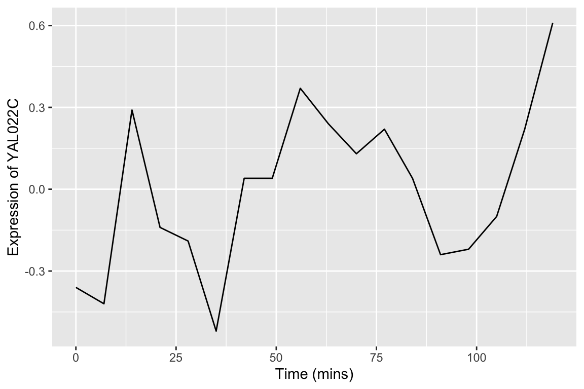
We can easily modify the above code block to visualize the expression of multiple genes of interest:
genes.of.interest <- c("YAL022C", "YAR018C", "YGR188C")

spellman.final |>
  filter(gene %in% genes.of.interest, expt == "alpha") |>
  ggplot(aes(x = time, y = expression, color = gene)) +
    geom_line() +
    labs(x = "Time (mins)", y = "Normalized expression",
         title = "Expression of multiple genes\nfollowing synchronization by alpha factor")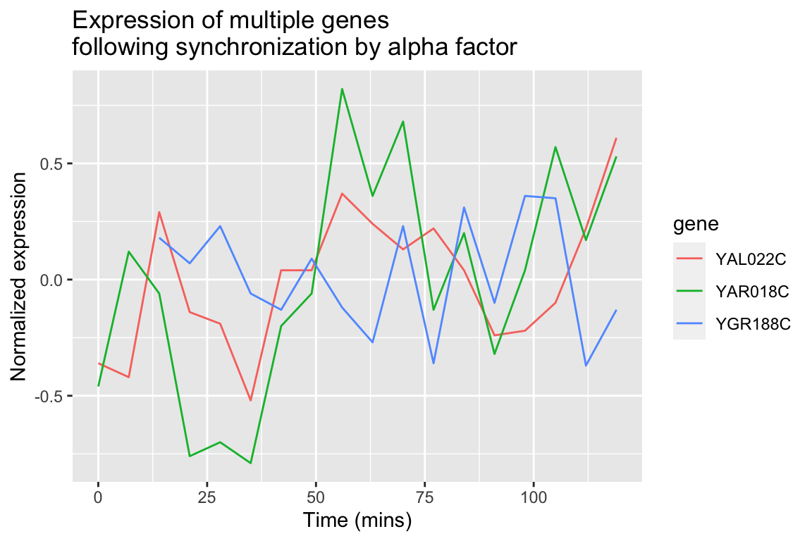
By employing facet_wrap() we can visualize the relationship between this set of genes in each of the experiment types:
spellman.final |>
  filter(gene %in% genes.of.interest) |>
  ggplot(aes(x = time, y = expression, color = gene)) +
    geom_line() +
    facet_wrap(~ expt) +
    labs(x = "Time (mins)", y = "Normalized expression",
title = "Expression of Multiple Genes\nAcross experiments") 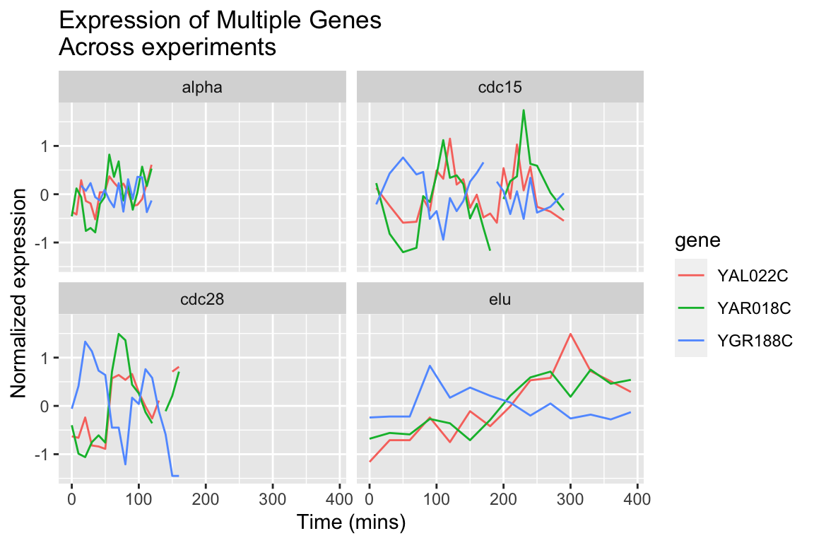
The different experimental treatments were carried out for varying lengths of time due to the differences in their physiological effects. Plotting them all on the same time scale can obscure that patterns of oscillation we might be interested in, so let’s modify our code block so that plots that share the same y-axis, but have differently scaled x-axes.
spellman.final |>
  filter(gene %in% genes.of.interest) |>
  ggplot(aes(x = time, y = expression, color = gene)) +
    geom_line() +
    facet_wrap(~ expt, scales = "free_x") +
    labs(x = "Time (mins)", y = "Normalized expression",
title = "Expression of Multiple Genes\nAcross experiments") 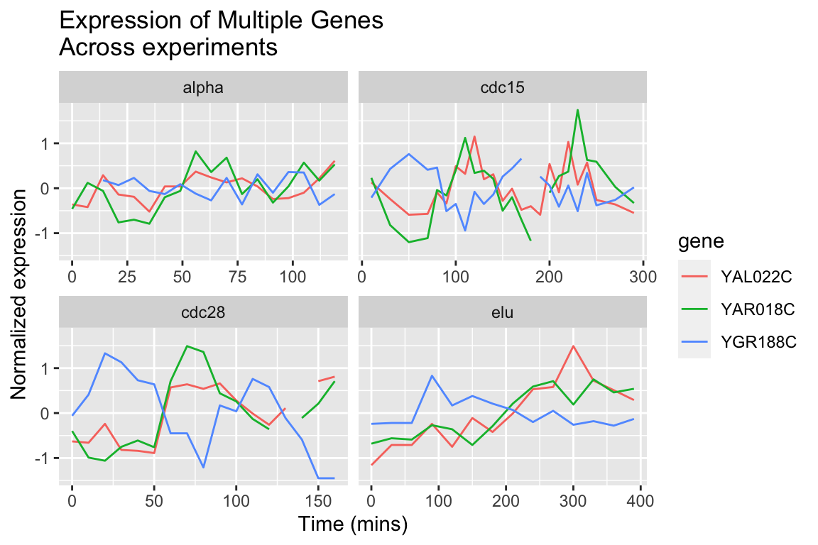
8.9.2 Finding the most variable genes
When dealing with vary large data sets, one ad hoc filtering criteria that is often employed is to focus on those variables that exhibit that greatest variation. To do this, we first need to order our variables (genes) by their variance. Let’s see how we can accomplish this using our long data frame:
by.variance <-
  spellman.final |>
  group_by(gene) |>
  summarize(expression.var = var(expression, na.rm = TRUE)) |>
  arrange(desc(expression.var))

head(by.variance)
## # A tibble: 6 × 2
##   gene    expression.var
##   <chr>            <dbl>
## 1 YLR286C           2.16
## 2 YNR067C           1.73
## 3 YNL327W           1.65
## 4 YGL028C           1.57
## 5 YHL028W           1.52
## 6 YKL164C           1.52
The code above calculates the variance of each gene but ignores the fact that we have different experimental conditions. To take into account the experimental design of the data at hand, let’s calculate the average variance across the experimental conditions:
by.avg.variance <-
  spellman.final |>
  group_by(gene, expt) |>
  summarize(expression.var = var(expression, na.rm = TRUE)) |>
  group_by(gene) |>
  summarize(avg.expression.var = mean(expression.var))
## `summarise()` has grouped output by
## 'gene'. You can override using the
## `.groups` argument.

head(by.avg.variance)
## # A tibble: 6 × 2
##   gene    avg.expression.var
##   <chr>                <dbl>
## 1 YAL001C              0.102
## 2 YAL002W              0.104
## 3 YAL003W              0.321
## 4 YAL004W              0.540
## 5 YAL005C              0.678
## 6 YAL007C              0.109
Based on the average experession variance across experimental conditions, let’s get the names of the 1000 most variable genes:
top.genes.1k <-
  by.avg.variance |>
  slice_max(avg.expression.var, n = 1000) |>
  pull(gene)

head(top.genes.1k)
## [1] "YFR014C" "YFR053C" "YBL032W" "YDR274C" "YLR286C" "YMR206W"
8.9.3 Heat maps
In our prior visualizations we’ve used line plots to depict how gene expression changes over time. For example here are line plots for 15 genes in the data set, in the cdc28 experimental conditions:
genes.of.interest <- c("YHR084W", "YBR083W", "YPL049C", "YDR480W",
                       "YGR040W", "YLR229C", "YDL159W", "YBL016W",
                       "YDR103W", "YJL157C", "YNL271C", "YDR461W",
                       "YHL007C", "YHR005C", "YJR086W")

spellman.final |>
  filter(expt == "cdc28", gene %in% genes.of.interest) |>
  ggplot(aes(x = time, y = expression, color=gene)) +
    geom_line() +
    labs(x = "Time (min)", y = "Expression")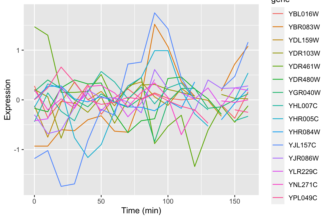
Even with just 10 overlapping line plots, this figure is quite busy and it’s hard to make out the individual behavior of each gene.
An alternative approach to depicting such data is a “heat map” which depicts the same information in a grid like form, with the expression values indicated by color. Heat maps are good for depicting large amounts of data and providing a coarse “10,000 foot view”. We can create a heat map using geom_tile as follows:
spellman.final |>
  filter(expt == "cdc28", gene %in% genes.of.interest) |>
  ggplot(aes(x = time, y = gene)) +
    geom_tile(aes(fill = expression)) +
    xlab("Time (mins)")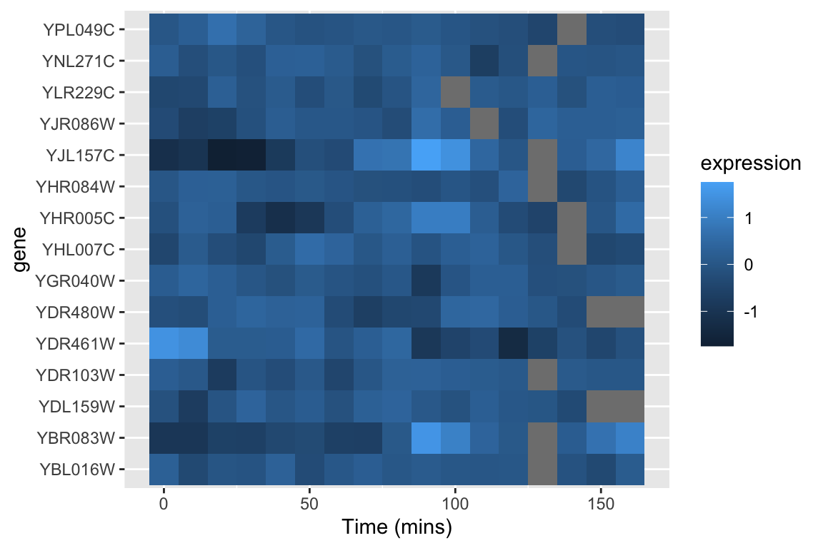
This figure represents the same information as our line plot, but now there is row for each gene, and the expression of that gene at a given time point is represented by color (scale given on the right). Missing data is shown as gray boxes. Unfortunately, the default color scale used by ggplot is a very subtle gradient from light to dark blue. This make it hard to distinguish patterns of change. Let’s now see how we can improve that.
8.9.3.1 Better color schemes with RColorBrewer
The RColorBrewer packages provides nice color schemes that are useful for creating heat maps. RColorBrewer defines a set of color palettes that have been optimized for color discrimination, many of which are color blind friendly, etc. Install the RColorBrewer package using the command line or the RStudio GUI.
Once you’ve installed the RColorBrewer package you can see the available color palettes as so:
library(RColorBrewer)

# show representations of the palettes
par(cex = 0.5) # reduce size of text in the following plot
display.brewer.all() 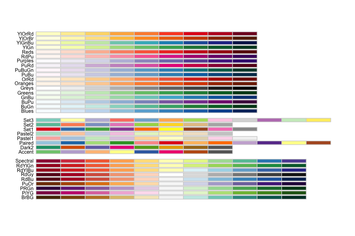
We’ll use the Red-to-Blue (“RdBu”) color scheme defined in RColorBrewer, however we’ll reverse the scheme so blues represent low expression and reds represent high expression. We’ll divide the range of color values into 9 discrete bins.
# displays the RdBu color scheme divided into a palette of 9 colors
display.brewer.pal(9, "RdBu") 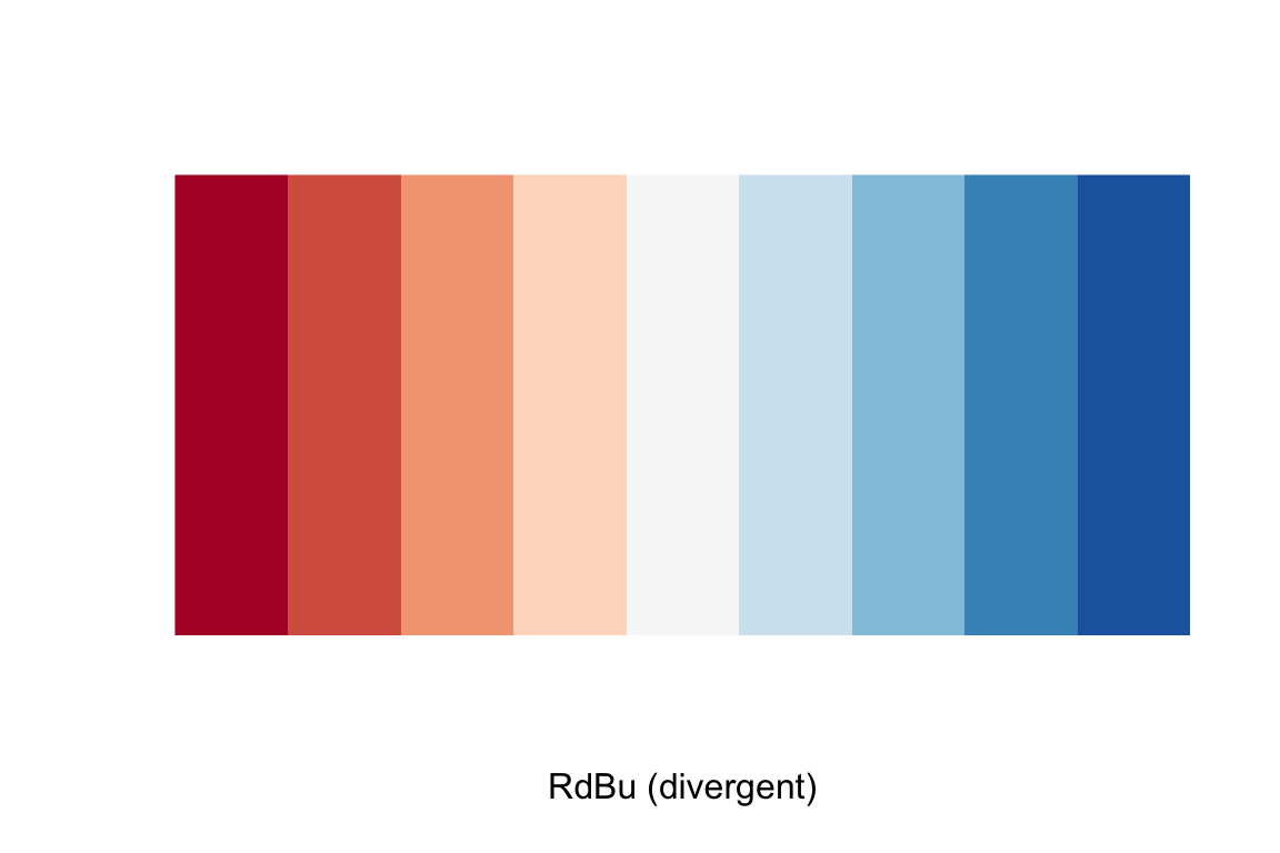
# assign the reversed (blue to red) RdBu palette
color.scheme <- rev(brewer.pal(9,"RdBu"))
Now let’s regenerate the heat map we created previously with this new color scheme. To do this we specify a gradient color scale using the scale_fill_gradientn() function from ggplot. In addition to specifying the color scale, we also constrain the limits of the scale to insure it’s symmetric about zero.
spellman.final |>
  filter(expt == "cdc28", gene %in% genes.of.interest) |>
  ggplot(aes(x = time, y = gene)) +
    geom_tile(aes(fill = expression)) +
    scale_fill_gradientn(colors=color.scheme,
                         limits = c(-2.5, 2.5)) +
    xlab("Time (mins)")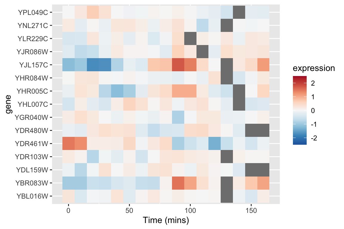
8.9.3.2 Looking for patterns using sorted data and heat maps
The real power of heat maps becomes apparent when you you rearrange the rows of the heat map to emphasize patterns of interest.
For example, let’s create a heat map in which we sort genes by the time of their maximal expression. This is one way to identify genes that reach their peak expression at similar times, which is one criteria one might use to identify genes acting in concert.
For simplicities sake we will restrict our attention to the cdc28 experiment, and only consider the 1000 most variables genes with no more than one missing observation in this experimental condition.
cdc28 <-
  spellman.final |>
  filter(expt == "cdc28") |>
  group_by(gene) |>
  filter(sum(is.na(expression)) <= 1) |>
  ungroup()   # removes grouping information from data frame

top1k.genes <-
  cdc28 |>
  group_by(gene) |>
  summarize(expression.var = var(expression, na.rm = TRUE)) |>
  slice_max(expression.var, n = 1000) |>
  pull(gene)

top1k.cdc28 <-
  cdc28 |>
  filter(gene %in% top1k.genes)
To find the time of maximum expression we’ll employ the function which.max (which.min), which finds the index of the maximum (minimum) element of a vector. For example to find the index of the maximum expression measurement for YAR018C we could do:
top1k.cdc28 |>
  filter(gene == "YAR018C") |>
  pull(expression) |>
  which.max()
## [1] 8
From the code above we find that the index of the observation at which YAR018C is maximal at 8. To get the corresponding time point we can do something like this:
max.index.YAR018C <-
  top1k.cdc28 |>
  filter(gene == "YAR018C") |>
  pull(expression) |>
  which.max()

top1k.cdc28$time[max.index.YAR018C]
## [1] 70
Thus YAR018C expression peaks at 70 minutes in the cdc28 experiment.
To find the index of maximal expression of all genes we can apply the dplyr::group_by() and dplyr::summarize() functions
peak.expression.cdc28 <-
  top1k.cdc28 |>
  group_by(gene) |>
  summarise(peak = which.max(expression))

head(peak.expression.cdc28)
## # A tibble: 6 × 2
##   gene       peak
##   <chr>     <int>
## 1 YAL003W      10
## 2 YAL005C       2
## 3 YAL022C      17
## 4 YAL028W       5
## 5 YAL035C-A    12
## 6 YAL038W      15
Let’s sort the order of genes by their peak expression:
peak.expression.cdc28 <- arrange(peak.expression.cdc28, peak)We can then generate a heatmap where we sort the rows (genes) of the heatmap by their time of peak expression. We introduce a new geom – geom_raster – which is like geom_tile but better suited for large data (hundreds to thousands of rows)
The explicit sorting of the data by peak expression is carried out in the call to scale_y_discrete() where the limits (and order) of this axis are set with the limits argument (see scale_y_discrete and discrete_scale in the ggplot2 docs).
# we reverse the ordering because geom_raster (and geom_tile)
# draw from the bottom row up, whereas we want to depict the
# earliest peaking genes at the top of the figure
gene.ordering <- rev(peak.expression.cdc28$gene)

top1k.cdc28 |>
  ggplot(aes(x = time, y = gene)) +
  geom_raster(aes(fill = expression)) +  #
  scale_fill_gradientn(limits=c(-2.5, 2.5),
                       colors=color.scheme) +
  scale_y_discrete(limits=gene.ordering) +
  labs(x = "Time (mins)", y = "Genes",
       title = "1000 most variable genes",
       subtitle = "Sorted by time of peak expression") +
  # the following line suppresses tick and labels on y-axis
  theme(axis.text.y = element_blank(), axis.ticks.y = element_blank())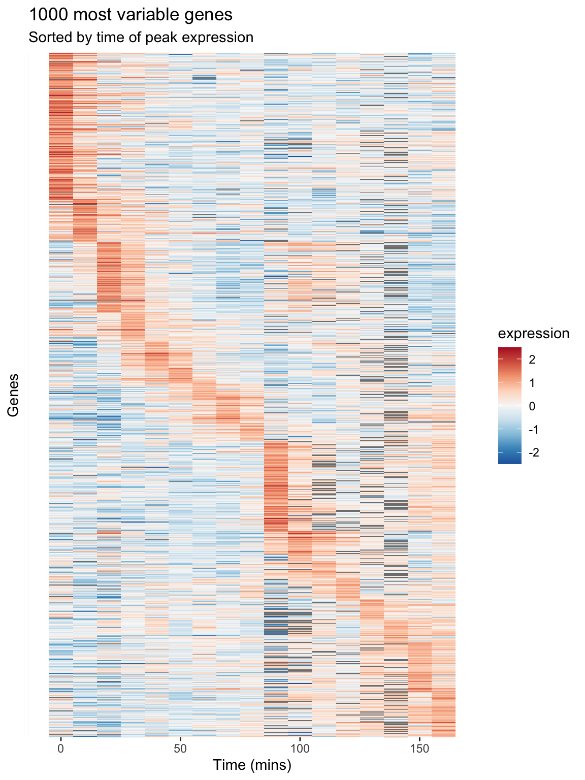
Figure 8.1: A Heatmap showing genes in the cdc28 experiment, sorted by peak expression
The brightest red regions in each row of the heat map correspond to the times of peak expression, and the sorting of the rows helps to highlight those gene whose peak expression times are similar.
8.10 Long-to-wide conversion using pivot_wider()
Our long data frame consists of four variables – gene, expt, time, and expression. This made it easy to create visualizations and summaries where time and expression were the primaries variables of interest, and gene and experiment type were categories we could condition on.
To facilitate analyses that emphasize comparison between genes, we want to create a new data frame in which each gene is itself treated as a variable of interest along with time, and experiment type remains a categorical variable. In this new data frame rather than just four columns in our data frame, we’ll have several thousand columns – one for each gene.
To accomplish this reshaping of data, we’ll use the function tidyr::pivot_wider(). tidyr::pivot_wider() is the inverse of tidyr::pivot_longer(). pivot_longer() took multiple columns and collapsed them together into a smaller number of new columns. By contrast, pivot_wider() creates new columns by spreading values from single columns into multiple columns.
Here let’s use pivot_wider to spread the gene name and expression value columns to create a new data frame where the genes are the primary variables (columns) of the data.
spellman.wide <-
  spellman.final |>
  select(-std.name, -description) |> # drop unneeded columns
  pivot_wider(names_from = gene, values_from = expression)
Now let’s examine the dimensions of this wide version of the data:
dim(spellman.wide)
## [1]   73 6180
And here’s a visual view of the first few rows and columns of the wide data:
spellman.wide[1:5, 1:8]
## # A tibble: 5 × 8
##   expt   time YAL001C YAL002W YAL003W YAL004W YAL005C YAL007C
##   <chr> <int>   <dbl>   <dbl>   <dbl>   <dbl>   <dbl>   <dbl>
## 1 alpha     0   -0.15   -0.11   -0.14   -0.02   -0.05   -0.6
## 2 alpha     7   -0.15    0.1    -0.71   -0.48   -0.53   -0.45
## 3 alpha    14   -0.21    0.01    0.1    -0.11   -0.47   -0.13
## 4 alpha    21    0.17    0.06   -0.32    0.12   -0.06    0.35
## 5 alpha    28   -0.42    0.04   -0.4    -0.03    0.11   -0.01
From this view we infer that the rows of the data set represent the various combination of experimental condition and time points, and the columns represents the 6178 genes in the data set plus the two columns for expt and time.
8.11 Exploring bivariate relationships using “wide” data
The “long” version of our data frame proved useful for exploring how gene expression changed over time. By contrast, our “wide” data frame is more convenient for exploring how pairs of genes covary together. For example, we can generate bivariate scatter plots depicting the relationship between two genes of interest:
two.gene.plot <-
  spellman.wide |>
  filter(!is.na(YAR018C) & !is.na(YAL022C)) |>  # remove NAs
  ggplot(aes(x = YAR018C, y = YAL022C)) +
    geom_point() +
    theme(aspect.ratio = 1)

two.gene.plot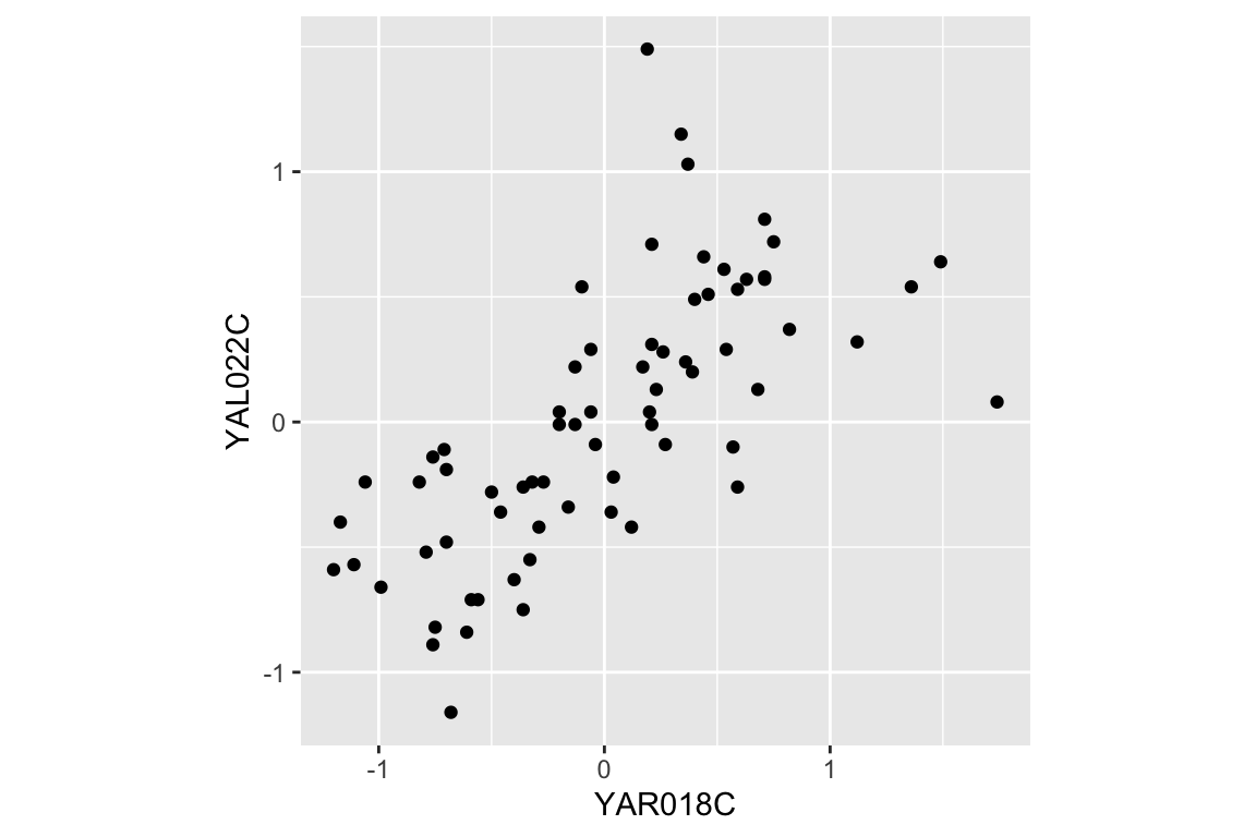
From the scatter plot we infer that the two genes are “positively correlated” with each other, meaning that high values of one tend to be associated with high values of the other (and the same for low values).
We can easily extend this visualization to facet the plot based on the experimental conditions:
two.gene.plot + facet_wrap(~expt, nrow = 2, ncol = 2) 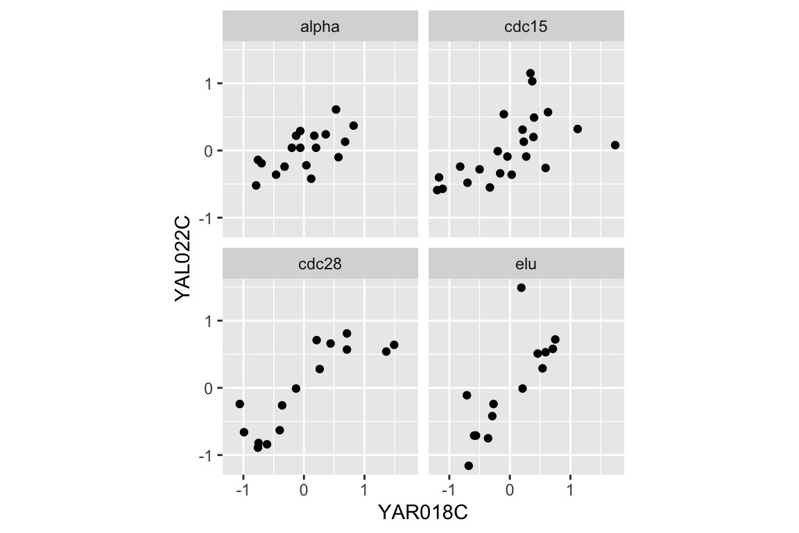
Correlation is a standard measure the degree of association between pairs of continuous variables. Briefly, correlation is a measure of linear association between a pair of variables, and ranges from -1 to 1. A value near zero indicates the variables are uncorrelated (no linear association), while values approaching +1 indicate a strong positive association (the variables tend to get bigger or smaller together) while values near -1 indicate strong negative association (when one variable is larger, the other tends to be small).
Let’s calculate the correlation between YAR018C and YAL022C:
spellman.wide |>
  filter(!is.na(YAR018C) & !is.na(YAL022C)) |>
  summarize(cor = cor(YAR018C, YAL022C))
## # A tibble: 1 × 1
##     cor
##   <dbl>
## 1 0.692
The value of the correlation coefficient for YAR018C and YAL022C, ~0.69, indicates a fairly strong association between the two genes.
As we did for our visualization, we can also calculate the correlation coefficients for the two genes under each experimental condition:
spellman.wide %>%
  filter(!is.na(YAR018C) & !is.na(YAL022C)) |>
  group_by(expt) |>
  summarize(cor = cor(YAR018C, YAL022C))
## # A tibble: 4 × 2
##   expt    cor
##   <chr> <dbl>
## 1 alpha 0.634
## 2 cdc15 0.575
## 3 cdc28 0.847
## 4 elu   0.787
This table suggests that the the strength of correlation between YAR018C and YAL022C may depend on the experimental conditions, with the highest correlations evident in the cdc28 and elu experiments.
8.11.1 Large scale patterns of correlations
Now we’ll move from considering the correlation between two specific genes to looking at the correlation between many pairs of genes. As we did in the previous section, we’ll focus specifically on the 1000 most variable genes in the cdc28 experiment.
First we filter our wide data set to only consider the cdc28 experiment and those genes in the top 1000 most variable genes in cdc28:
top1k.cdc28.wide <-
  top1k.cdc28 |>
  select(-std.name, -description) |>
  pivot_wider(names_from = gene, values_from = expression)
With this restricted data set, we can then calculate the correlations between every pair of genes as follows:
cdc28.correlations <-
  top1k.cdc28.wide |>
  select(-expt, -time)  |> # drop expt and time
  cor(use = "pairwise.complete.obs")
The argument use = "pairwise.complete.obs" tells the correlation function that for each pair of genes to use only the pariwse where there is a value for both genes (i.e. neither one can be NA).
Given \(n\) genes, there are \(n \times n\) pairs of correlations, as seen by the dimensions of the correlation matrix.
dim(cdc28.correlations)
## [1] 1000 1000
To get the correlations with a gene of interest, we can index with the gene name on the rows of the correlation matrix. For example, to get the correlations between the gene YAR018C and the first 10 genes in the top 1000 set:
cdc28.correlations["YAR018C",1:10]
##     YAL003W     YAL005C     YAL022C     YAL028W   YAL035C-A     YAL038W
##  0.07100626 -0.53315493  0.84741624  0.33379901 -0.22316755 -0.03984599
##     YAL044C     YAL048C     YAL060W     YAL062W
##  0.32253692  0.12220221  0.49445700 -0.60972118
In the next statement we extract the names of the genes that have correlations with YAR018C greater than 0.6. First we test genes to see if they have a correlation with YAR018C greater than 0.6, which returns a vector of TRUE or FALSE values. This vector of Boolean values is than used to index into the row names of the correlation matrix, pulling out the gene names where the statement was true.
pos.corr.YAR018C <- rownames(cdc28.correlations)[cdc28.correlations["YAR018C",] > 0.6]
length(pos.corr.YAR018C)
## [1] 65
We then return to our long data to show this set of genes that are strongly positively correlated with YAR018C.
top1k.cdc28 |>
  filter(gene %in% pos.corr.YAR018C) |>
  ggplot(aes(x = time, y = expression, group = gene)) +
    geom_line(alpha = 0.33) +
    theme(legend.position = "none")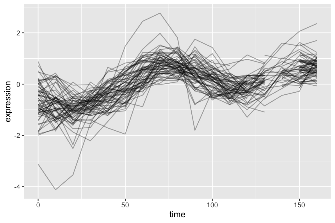
As is expected, genes with strong positive correlations with YAR018C show similar temporal patterns with YAR018C.
We can similarly filter for genes that have negative correlations with YAR018C.
neg.corr.YAR018C <- colnames(cdc28.correlations)[cdc28.correlations["YAR018C",] <= -0.6]As before we generate a line plot showing these genes:
top1k.cdc28 |>
  filter(gene %in% neg.corr.YAR018C) |>
  ggplot(aes(x = time, y = expression, group = gene)) +
    geom_line(alpha = 0.33) +
theme(legend.position = "none") 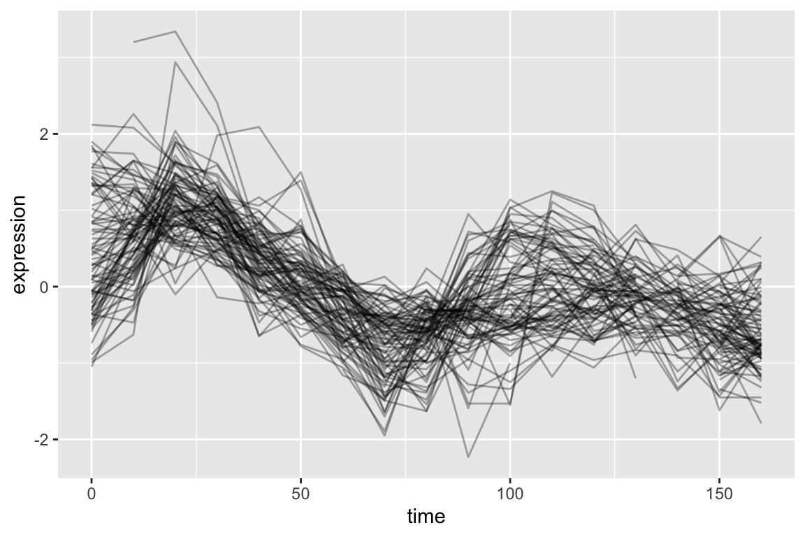
8.11.2 Adding new columns and combining filtered data frames
Now let’s create a new data frame by: 1) filtering on our list of genes that have strong positive and negative correlations with YAR018C; and 2) creating a new variable, “corr.with.YAR018C”, which indicates the sign of the correlation. We’ll use this new variable to group genes when we create the plot.
pos.corr.df <-
  top1k.cdc28 |>
  filter(gene %in% pos.corr.YAR018C) |>
  mutate(corr.with.YAR018C = "positive")

neg.corr.df <-
  top1k.cdc28 |>
  filter(gene %in% neg.corr.YAR018C) |>
  mutate(corr.with.YAR018C = "negative")

combined.pos.neg <- rbind(pos.corr.df, neg.corr.df)
Finally, we plot the data, colored according to the correlation with YAR018C:
ggplot(combined.pos.neg,
       aes(x = time, y = expression,  group = gene,
           color = corr.with.YAR018C)) +
  geom_line(alpha=0.25) +
  geom_line(aes(x = time, y = expression),
            data = filter(top1k.cdc28, gene == "YAR018C"),
            color = "DarkRed", size = 2,alpha=0.5) +
  # changes legend title and values for color sclae
  scale_color_manual(name = "Correlation with YAR018C",
                       values = c("blue", "red"))  +
  labs(title = "Genes strongly positively and negatively correlated with YAR018C",
       subtitle = "YAR018C shown in dark red",
       x = "Time (mins)", y = "Expression")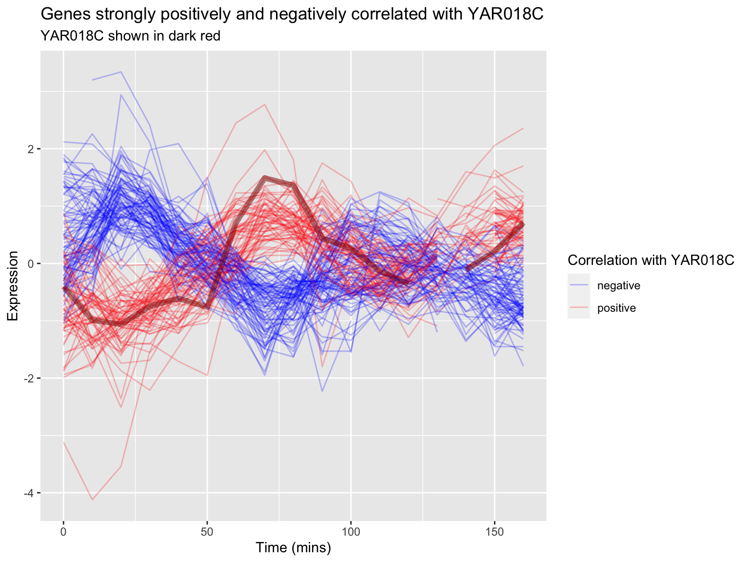
8.11.3 A heat mapped sorted by correlations
In our previous heat map example figure, we sorted genes according to peak expression. Now let’s generate a heat map for the genes that are strongly correlated (both positive and negative) with YAR018C. We will sort the genes according to the sign of their correlation.
# re-factor gene names so positive and negative genes are spatially distinct in plot
combined.pos.neg$gene <-
  factor(combined.pos.neg$gene,
         levels = c(pos.corr.YAR018C, neg.corr.YAR018C))

combined.pos.neg |>
  ggplot(aes(x = time, y = gene)) +
    geom_tile(aes(fill = expression)) +
    scale_fill_gradientn(colors=color.scheme) +
    xlab("Time (mins)")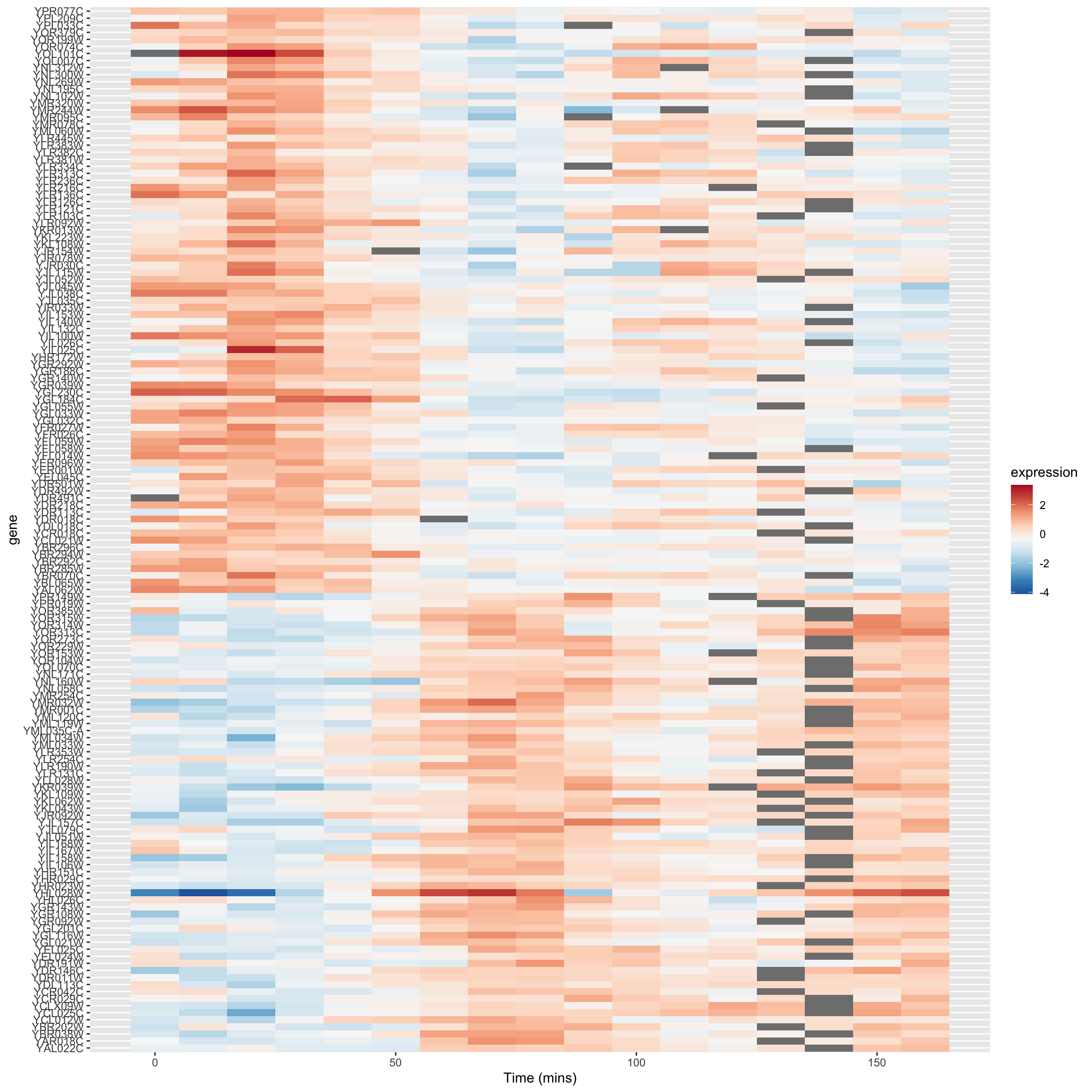
The breakpoint between the positively and negatively correlated sets of genes is quite obvious in this figure.
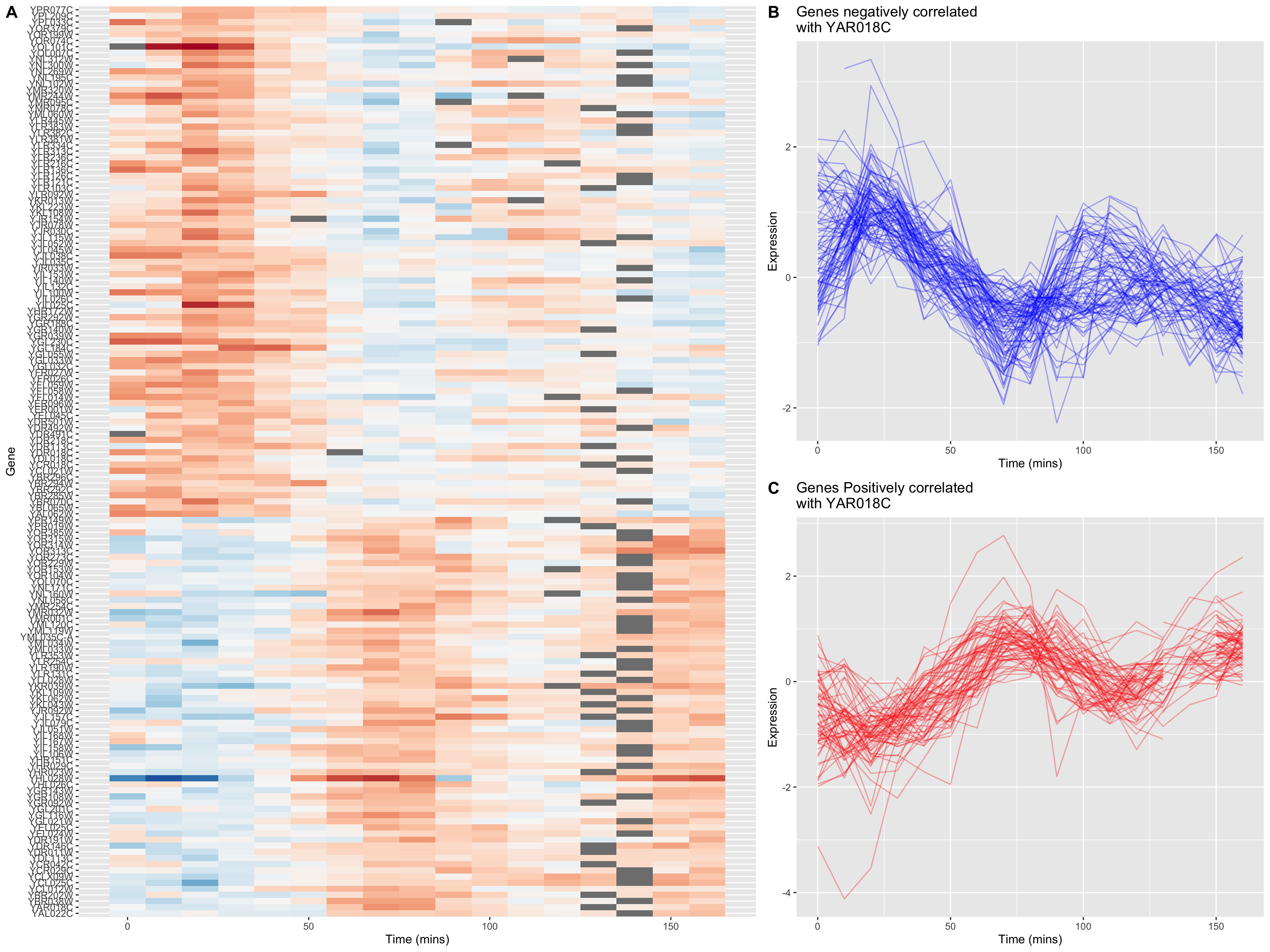
8.11.4 A “fancy” figure
Recall that we introduced the cowplot library in Chapter 6, as a way to combine different ggplot outputs into subfigures such as you might find in a published paper. Here we’ll make further use cowplot to combine our heat map and line plot visualizations of genes that covary with YAR018C.
library(cowplot)cowplot’s draw_plot() function allows us to place plots at arbitrary locations and with arbitrary sizes onto the canvas. The coordinates of the canvas run from 0 to 1, and the point (0, 0) is in the lower left corner of the canvas. We’ll use draw_plot to draw a complex figure with a heatmap on the left, and two smaller line plots on the right.
pos.corr.lineplot <-
  combined.pos.neg |>
  filter(gene %in% pos.corr.YAR018C) |>
  ggplot(aes(x = time, y = expression, group = gene)) +
    geom_line(alpha = 0.33, color = 'red') +
    labs(x = "Time (mins)", y = "Expression",
      title = "Genes Positively correlated\nwith YAR018C")

neg.corr.lineplot <-
  combined.pos.neg |>
  filter(gene %in% neg.corr.YAR018C) |>
  ggplot(aes(x = time, y = expression, group = gene)) +
    geom_line(alpha = 0.33, color = 'blue') +
    labs(x = "Time (mins)", y = "Expression",
      title = "Genes negatively correlated\nwith YAR018C")


heat.map <-
  ggplot(combined.pos.neg, aes(x = time, y = gene)) +
    geom_tile(aes(fill = expression)) +
    scale_fill_gradientn(colors=color.scheme) +
    labs(x = "Time (mins)", y = "Gene") +
    theme(legend.position = "none")
The coordinates of the canvas run from 0 to 1, and the point (0, 0) is in the lower left corner of the canvas. We’ll use draw_plot to draw a complex figure with a heatmap on the left, and two smaller line plots on the right.
I determined the coordinates below by experimentation to create a visually pleasing layout.
fancy.plot <- ggdraw() +
  draw_plot(heat.map, 0, 0, width = 0.6) +
  draw_plot(neg.corr.lineplot, 0.6, 0.5, width = 0.4, height = 0.5) +
  draw_plot(pos.corr.lineplot, 0.6, 0,   width = 0.4, height = 0.5) +
  draw_plot_label(c("A", "B", "C"), c(0, 0.6, 0.6), c(1, 1, 0.5), size = 15)

fancy.plot